If I’m rolling a die and taking the mean I want to know what to expect. Maybe I don’t trust analysis and I’m not hugely patient.
Let’s use R to roll a die and see what we get:
d <- 1:6
sample(d, 1, replace='T')
I got a ‘1’. Yours might be different. Let’s try again: 4. Then 1, 2 and 5. So what’s the mean?
mean(c(1,4,1,2,5))
It’s 2.6. From this result, when a die is rolled, I should expect it to be 2.6.
Let’s try that again:
roll <- function(count, d = 1:6) {
  sample(d, count, replace='T')
}

mean(roll(5))
This time it’s 4.2. That’s different. What if we repeat this trial a few times?
hist(replicate(100, mean(roll(5))), xlim=c(0,6), xlab='Sample mean', main='Histogram of Sample Means')
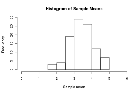
So I should expect the mean to be something between 2 and 5. But, if a single roll varies wildly, and a run of five less so, what if I increase my sample size? We still perform 100 trials, but each trial is now over a hundred rolls rather than five:
hist(replicate(100, mean(roll(100))), xlim=c(0,6), xlab='Sample mean', main='Histogram of Sample Means.')
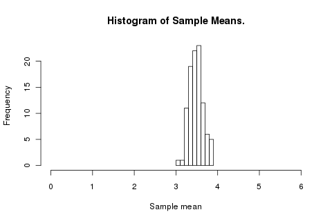
The mean isn’t changing but the variance is decreasing. How does the trend look? For each number of rolls 1 to 200 (every fourth number) we run that trial 4,000 times and make a box plot of the distribution of results.
As we continue to increase the number of rolls in a trial we can see the outliers start to move in:
sizes <- rep(seq(1, 200, 4), 4000)
plot(factor(sizes), sapply(sizes, function(x){mean(roll(x))}), xlab='Rolls', ylab='Distribution', ylim=c(0, 6))

By the time we’re rolling 100 times before calling the average we can be extremely confident that our result will lie between 2.5 and 4.5.
plot(1:1000, sapply(1:1000, function(x){mean(roll(x))}), ylim=c(0, 6), ylab='Mean', xlab='Rolls', type='p', pch=3)

Analytically, the expected value of a single roll of a die is simple enough:
It’s exactly 3.5. But, as this shows, the mean of a series of rolls will only tend to that value.
(Experimental investigation can mislead with pathological cases;
consider a
Black Swan
die: roll(10, d = append(rep(0, 999999), 1000000)).)
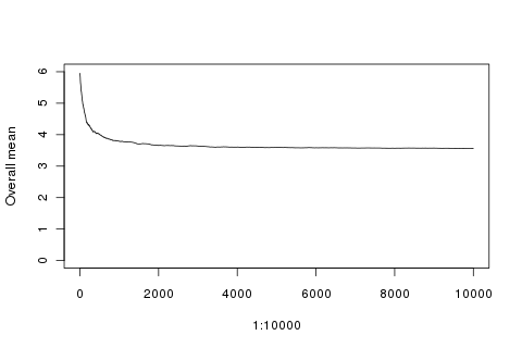
As a demonstration of regression to the mean, consider a fair die that’s just (inexplicably) rolled a hundred sixes in a row. For regression to the mean we’d expect the mean (currently six) to decrease as we keep rolling. So does that mean that it’s run out of sixes? No, just that, as the sample size increases, those intial rolls become less significant. Let’s plot the running mean:
rolls <- roll(10000)
plot(1:10000, sapply(1:10000, function(x){mean(append(rep(6, 100), rolls[1:x]))}), type='l', ylim=c(0, 6), ylab='Overall mean')
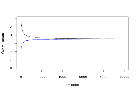
And if that lucky initial run had been all 2s?
points(1:10000, sapply(1:10000, function(x){mean(append(rep(2, 100), rolls[1:x]))}), type='l', ylim=c(0, 6), ylab='Overall mean', col='blue')
(Better check those rolls look reasonable: plot(factor(rolls)).)
Those are just two possible sequences after the inital runs. It’s possible that, even for a fair die, we’d continue to get more sixes. Let’s keep rolling, again and again, and take the run with the highest mean.
m <- 0
for (x in 1:10000) {
  nr <- roll(1000)
  nm <- mean(nr)
  if (nm > m) {
    m <- nm; r <- nr;
  }
}

plot(1:1000, sapply(1:1000, function(x){mean(append(rep(6, 100), r[1:x]))}), type='l', ylim=c(0, 6), ylab='Mean', xlab='Rolls')

For comparison, let’s take the lowest run and also the expected mean:
plot(1:1000, sapply(1:1000, function(x){mean(append(rep(6, 100), r[1:x]))}), type='l', ylim=c(0, 6), ylab='Mean', xlab='Rolls', col='red')

m <- 6
for (x in 1:10000) {
  nr <- roll(1000)
  nm <- mean(nr)
  if (nm < m) {
    m <- nm; r <- nr;
  }
}

points(1:1000, sapply(1:1000, function(x){mean(append(rep(6, 100), r[1:x]))}), type='l', ylim=c(0, 6), ylab='Mean', xlab='Rolls', col='blue')

points(1:1000, sapply(1:1000, function(x){mean(append(rep(6, 100), rep(3.5, x)))}), type='l', ylim=c(0, 6), ylab='Mean', xlab='Rolls', col='black')
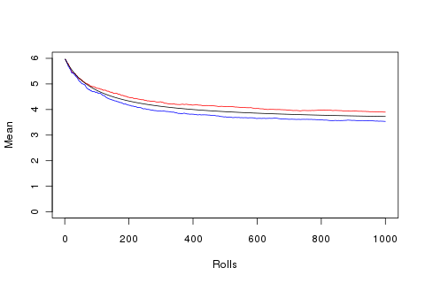
So ten thousand attempts to get the best and worst sequence of 1000 rolls adds up to not a huge difference.
It’s easy (and fun) to misuse statistics. There are also plenty of concepts, great results, and reminders of orders of magnitude to learn from, and R is a great tool for quick experimentation.